Create value from data on the road to autonomous manufacturing

29 April 2020

Big Data hype continues to permeate our lives and all companies feel the pressure to act quickly and stay competitive. In pharma manufacturing, this means optimized production facilities fully controlled by Artificial Intelligence (AI) – also known as autonomous manufacturing. But value creation in this area is not always clear, especially short-term.

To tackle these uncertainties, this article focuses on using data to create value and improving Overall Equipment Efficiency (OEE) in pharma manufacturing facilities. Using a seven-step road map, we describe in detail the first two steps and discuss where to make early savings.

Read the full article or follow the links to find each section:

• A seven-step road map towards autonomous manufacturing
• Intelligent use of data to reduce manufacturing costs
• Step one: How to reduce Quality Control costs
• Step two: How to rapidly map OEE improvement potential and identify changes
• OEE definitions

A seven step roadmap towards autonomous manufacturing

The illustration below shows a road map for reaching autonomous production with a focus on data analysis.

 

 

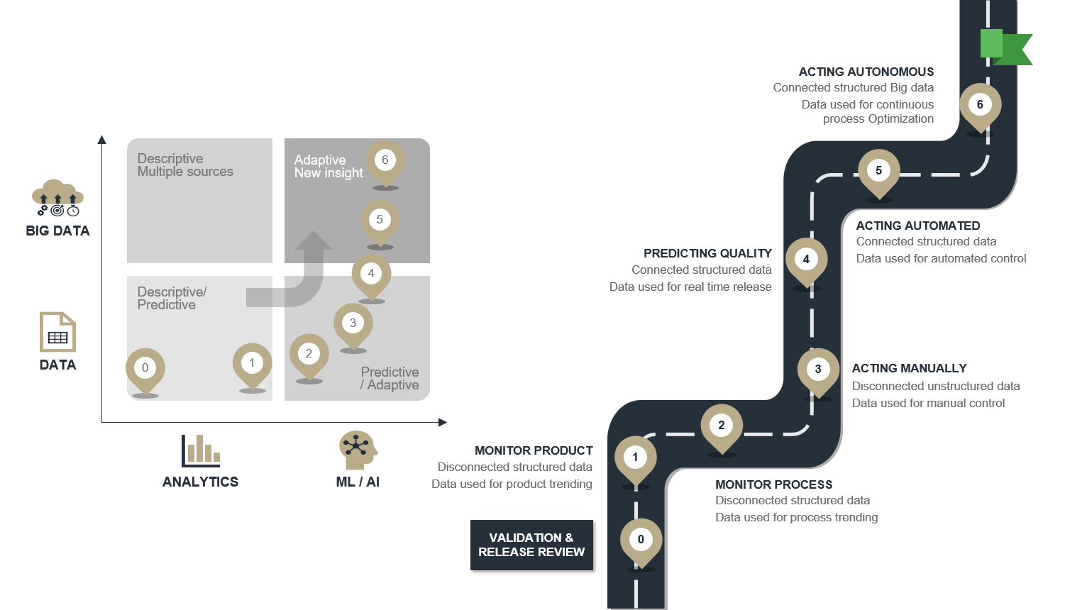
1. Review and reduce current Quality Control costs
2. Monitor product performance across batches to catch trends and map improvement potential
3. Monitor the process instead of the product to get faster feedback and ease diagnosis
4. Control the process by manually acting on what is monitored in step 2.
5. Predict the quality based on what is monitored in step 2 and model its relationship to quality to allow for real-time release testing
6. Act automated - based on automating step 3 and using knowledge from step 4.
7. Act autonomous - where models from step 4 and control patterns from step 5 are continuously optimized by AI.

 

Intelligent use of data to reduce pharma manufacturing costs

Cost reduction is a key focus area for most manufacturing companies. So how can the intelligent use of data help?

An obvious place to create value is to reduce the Full Manufacturing Cost per manufactured unit (FMCU). FMCU is simply the Total Costs (TC) divided by the released volume (V):

 

 

The volume (V) can be different units, including:

• Number of doses (up and down stream processing)
• Number of parts (medical device)
• Number of tablets

The importance of reducing quality control and non-conformity costs

How do you work out the total cost? The intelligent use of data is particularly relevant when considering the cost of Quality Control (QC) and Non-Conformity (NC). The calculation for TC is as follows:

Other costs include raw materials, consumables, depreciation, salary and services. And although the intelligent use of data can reduce these, the focus is this article is on QC and NC cost reductions.

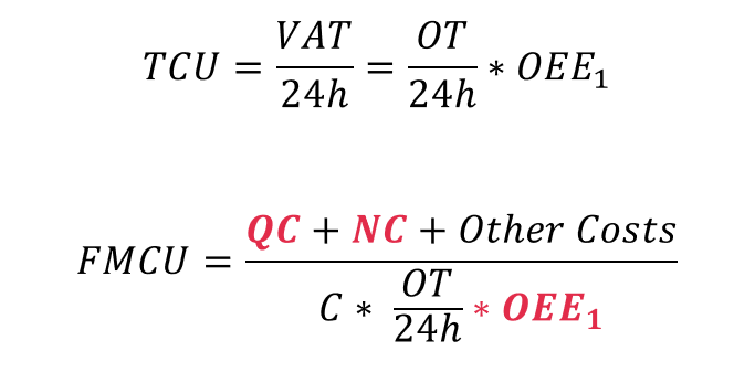
Reduce costs by increasing Total Capacity Utilization (TCU)

The volume (V) depends on the equipment capacity (C) and how well it is utilized. This is called Total Capacity Utilization (TCU). The calculation is as follows:

When focusing on cost reduction, the aim is to not increase capacity (which always comes with a cost) but increase the use of what you already have, i.e. increase TCU instead.

TCU and overall equipment efficiency (OEE)

There are many reasons for a low TCU. These can be described using OEE indices. Intelligent use of data will mainly contribute to increasing OEE₁. So, we will rewrite the equation to become:

 

 

Where OT is the Operating Time. For definitions of OEE indices, see the last section.

Now we have the calculations established, in the following section we describe the first two steps on the road map - how to reduce quality control and non-conformity costs and increase OEE1 with the intelligent use of data.

 

Step one: How to reduce Quality Control costs

How it is done today

In traditional pharmaceutical production, we inspect the final product quality by sampling it as a part of batch release. This can be a very costly process, due to:

• Large sample sizes
• The many quality attributes that need to be measured
• High testing costs

Often, companies use AQL sampling standards like ISO2859 (Go/NoGo testing) or ISO3951 (continuous variables), which leads to large sample sizes and poor customer protection.

The purpose of AQL sampling is to ensure a batch with an error rate at AQL has a high probability of passing the test. In addition, AQL no longer means Acceptable Quality Level but Acceptance Quality Limit, i.e. to which level we have tested.

Typically, AQL is much higher than the error rate a customer would find acceptable. This combination leads to poor consumer protection.

How it should be done in the future

Instead, we should prove with confidence that the batch is even better than the quality the consumer would find acceptable (the original definition of AQL). If what we are making is good quality, there is a large margin between what we can do and what the customer can accept. This leaves space for estimation uncertainty on quality level, which means low sample sizes and ultimately lower costs.

The illustration below shows a road map to reduce QC costs:

 

 

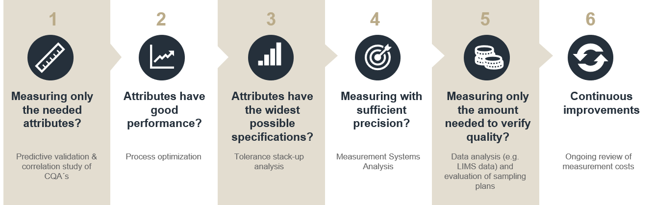
To ensure a large margin between what you can do and the acceptance criteria, you must ensure:

• You have good quality performance.
• You make the specifications as wide as possible. Safety margins are NOT needed since we enforce with confidence.
• You have good measurement performance, so poor measurement precision does not reduce the gap. Often stricter requirements in Measurement Method Validation are needed.

Sample sizes can be further reduced with intelligent data analysis:

• Make correlation studies between quality attributes to see if some can be predicted by others, and therefore remove the need to measure everything.
• Instead of running the same large sample size every day (which must work even on a bad day), use sequential sampling, where you test samples only until you can prove quality with confidence.
• Use historical data, e.g. validation data to estimate variation with confidence. This way you only need to estimate mean values with confidence in production samples. This requires much lower sample sizes than standard deviations
• Describe data with a model across parallel production units, product types, sampling points and batches instead of stratifying data into smaller data sets that are analyzed individually. From this model, future batch (validation) or untested products (batch release) performance can be predicted with confidence using prediction intervals.

A case example of quality control cost reductions

Combining these techniques often leads to much smaller sample sizes than the ones currently used. Figure 4 shows how the last two bullet points above can be used to reduce the sample size in batch release (in this case, from 27 to 3).

The following is illustrated in the graph below:

Y-axis:

• Specification limits (blue lines)
• Narrowed specification limits for means based on historical data (dotted blue lines)
• Prediction limits for means based on historical data(red)
• Target (green)

X-axis:

• Number (N) if observations

If a mean of observations is inside the narrowed specification limits (dotted blue) the batch can be released. This is because we have proven that there is less than AQL risk (in the shown case 0.135%) that untested parts will be outside specifications.

When the prediction limits (red) are outside narrowed specification lines (dotted blue) there is more than β risk (in the shown case 5%) that we cannot release the batch based on a sample size of N. In the shown case, we need a sample size of 3 before the red lines are inside the dotted blue.

 

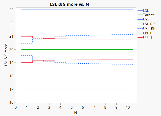
Above graph: Sample size calculation based on within batch variance from historical data.

By reducing the sample sizes, this alone reduces the risk of a Non-Conformity. In addition, by enlarging tolerances and ensuring that measurement systems are adequate to release within tolerances, we can remove NCs that are due to too large safety margin in tolerances and bad measurement precision respectively.

 

Step two: How to rapidly map OEE1 improvement potential and identify changes

Mapping potential before making an investment

Before investing and moving towards autonomous manufacturing, it is important to identify the improvement potential of OEE1 (speed/yield/recovery%). Collecting historical OOE1 data is normally possible within a few days, as shown below.

 

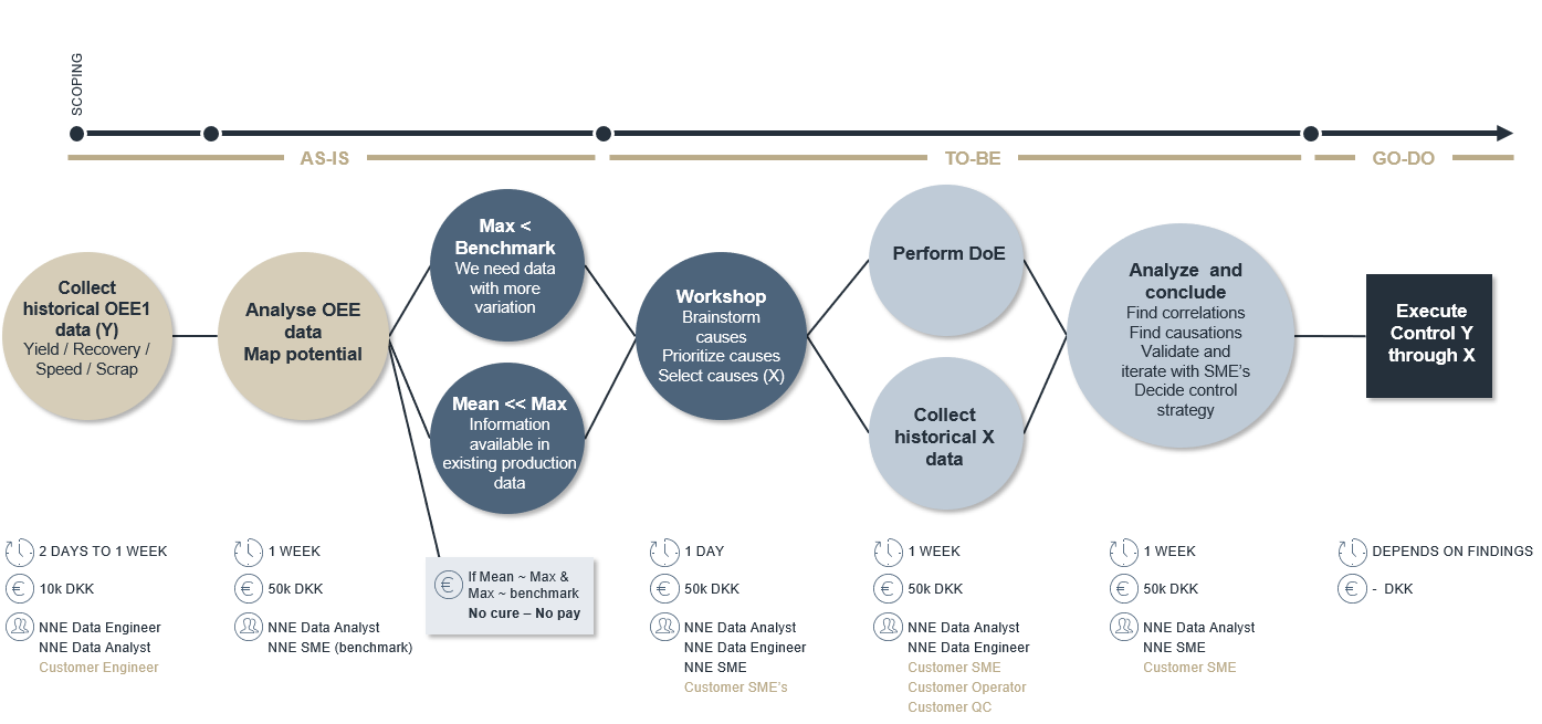
Above illustration: Rapid identification of improvement potential

To analyze this data, the questions are simple:

• What is the max OEE1?
• What is the mean and/or median OEE1?

From this, the following three scenarios are possible:

1. Max OEE1 is lower than the benchmark OEE1 (what other companies can do with similar processes). In this scenario, you cannot expect to find a solution in your historical data. You need to change your method, and need new data by making, for example, a Design of Experiments (DoE).
2. Max OEE1 is comparable to the benchmark but the mean/median OEE1 is much lower. There will be information in your historical data on how to stabilize your process at maximum OEE1.
3. Max OEE1 is comparable to benchmark OEE1 and mean/median OEE1 is close to Max OEE1. You should be happy with this result.

The cost reduction potential in either increasing mean OEE1 to Benchmark OEE1 or to Max OEE1 is straight forward.

Identify changes

In scenario 1 or 2, we need to identify variables to make a DoE (scenario 1) or collect data (scenario 2). Since this is not free of charge, we need to build on existing knowledge to identify these variables. This can be done through a 1-day workshop with process experts.

After prioritizing variables from the workshop, you should perform a DoE (scenario 1) or collect historical data (scenario 2). A model should be built on this data predicting what should be done and what would be obtained by either changing the method or stabilizing the process settings. The overall outcome will be the basis for a control strategy for production.

Implement findings

Finally, there is implementation. The time it takes to implement your findings is strongly dependent on outcomes(illustrated in the dark blue box above), but the time to identify potential findings is only a few weeks (sand coloured circles). This is the same for identifying actions to improve (seen in the blue and light blue circles).

 

OEE definitions

There are many reasons for a low TCU which can be described using OEE indices. It can relate to losses such as:

1. The factory is closed for too long or too many times in a period. E.g. unmanned shifts, holidays and weekends.
2. The production line and/or personnel are not available even though the factory is open. E.g. due to non-production activities like overall maintenance, sickness, training, and meetings.
3. Even though production lines and personnel are available, a lot of time is spent on batch specific non-production activities like change overs, line clearance and cleaning. This is the typical focus of Lean.
4. Even though the production line is operating, there are losses during operation compared to validated speed, e.g. speed and scrap loss. Speed loss is part production, typically short stops on the line. For upstream and downstream processes, it is typically low yields or recovery. Scrap loss are products that needs to be scrapped or reworked to pass QC tests.

The above-mentioned losses can be described by TCU and Overall Equipment Efficiency (OEE) indices. These indices are all ratios, where Value Adding Time (VAT) is the numerator.

VAT is defined as the ratio between how much was released per time unit (e.g. day) divided by validated speed/yield/recovery. In other words, how quickly could something be produced under ideal conditions in infinite batch sizes.

 In the denominator, we have different times:

• Calendar Time (24h)
• Manned Time (MT)
• Production Time (PT)
• Operation Time (OT)

Typically, three OEE indices are used on top of TCU:

 

 

The different OEE indices are shown below.

 

 

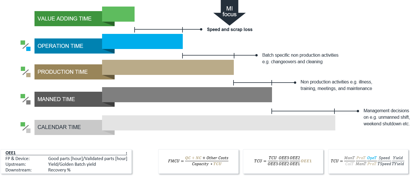
• OEE₃ describes the total efficiency of the manufacturing site taking loss 2-4 into consideration. This is typically how a site manager’s performance is measured. However, OOE 3 should only be high on bottleneck processes, otherwise non-bottleneck processes will be producing stock (which is not Lean).
• OEE₂ describes the efficiency of production, taking loss 3 and 4 into consideration. This is typically how a production manager’s performance is measured. As for OEE_3, it should only be high on bottleneck processes.
• OEE₁ describes the efficiency of the core production operation, taking only loss 4 into consideration. It should always be high, no matter the process.

Although intelligent manufacturing can be used to reduce all losses, it is ideal for reducing loss 4 and improving OEE1.

Finally, TCU and FMCU can be calculated as:

 

 

For more information, please contact Per Vase on PRVA@nne.com